Scientific Background

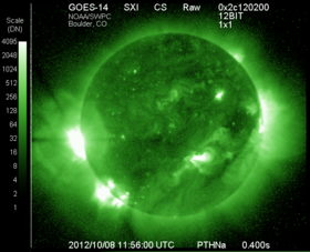
When a solar flare occurs on Sun (picture beside is taken by the GOES 14 satellite on October 8th, 2012 around noon UTC) a blast of intense ultraviolet and x-ray radiation hits the dayside of the Earth after a propagation time of about 8 minutes. This high energy radiation is absorbed by atmospheric particles, raising them to excited states and knocking electrons free in the process of photoionization. The low altitude ionospheric layers (D and E region) immediately increase in density over the entire dayside. The ionospheric disturbance enhances VLF radio propagation. Scientists on the ground can use this enhancement to detect solar flares; by monitoring the signal strength of a distant VLF transmitter, sudden ionospheric disturbances (SID) are recorded and indicate when solar x-ray flares have taken place. This high energetic radiation shall not be misstaken by the particle flux (the solar wind) travelling for several daysfrom the Sun after being ejected by an so-called coronal mass ejection. Solar wind particles travel usually with velocities of about 400 km/second and reaching Earth usually within some days. They in turn are cause for phenomena such as the aurora and can disturb ionosphere (E and F Region) and communication at high latitudes.

To understand the SID effect it is essential to remember how Earths' ionosphere is created and strucutred. One may see the the ionosphere as a shell of electrons and electrically charged ions (atoms and molecules) that surrounds the Earth, stretching from a height of about 60 km to more than 1,000 km. The main consituents of the ionsphere are neutral atoms and molecules. However, the charged nature of the ionosphere is due to production of plasma (electrons, ions) primarily by solar ultraviolet radiation. This again means that the ionosphere is 'produced' during the day and is 'reduced' during the night due to recombination processes of electrons and ions. Ionization depends primarily on the Sun and its activity. The amount of ionization in the ionosphere varies greatly with the amount of radiation received from the Sun.

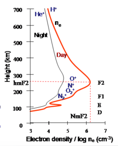
The structure of the ionosphere (layers or regions) is related to the neutral gas species populating those regions and the kinetic energy of the radiation penetrating into Earths' upper atmosphere. The higher energized the radiation is the lower it may penetrate and produce electrons and ions. The electron density profile (beside) shows the different ionospheric regions during day (production of electrons) and night (recombination of electrons). Effects related to terrestrial radio communication (ionospheric- or sky-waves) are due to the existence of the D and E-region - also called Kennelly–Heaviside layer. Ionospheric disturbances of the F-layer are commonly influencing global navigation satellite system (GNSS) communications and may coincide with the SID phenomena.

When Sun is active, strong solar flares can occur that will hit the sunlit side of Earth with hard X-rays. The X-rays will penetrate to the D-region, releasing electrons that will rapidly increase absorption, causing a High Frequency (3 - 30 MHz) radio blackout. During this time Very Low Frequency (3 – 30 kHz) signals will be reflected by the D layer instead of the E layer, where the increased atmospheric density will usually increase the absorption of the wave and thus dampen it. As soon as the X-rays end, the sudden ionospheric disturbance (SID) or radio black-out ends as the electrons in the D-region recombine rapidly and signal strengths return to normal.

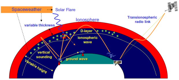
Above Figure sketches Earths' upper atmosphere, ground based instrumentations (radio transmitters, sounders and radio receivers), space instrumentation (satellites) as well as waves propagations. Earth ionosphere is a variable system with a variable thickness and electron distribution (profile) depending on spaceweather events (solar activiy, e.g. solar x-ray flares). Radio communication can be summerized as follows:

• short distance communication (ground wave, for distances ca. 800 km and less)
• long distance communication (skywave or ionospheric waves for intercontinental communcations)
• local ionospheric sounding (by ionospheric sounders, e.g. ionosondes and incoherent scatter radars)
• GNSS and satellite communication (via transionsopheric radio link - crossing the ionosphere)

Ionospheric radio waves (sky waves) are constantly modified in their amplitude, phase, orientation and polarization based on their frequency and the ionospheric conditions.

Short wave radio waves (in the HF range) are absorbed by the increased particles in the low altitude ionosphere causing a complete blackout of radio communications. This is called a short wave fading. These fadeouts last for a few minutes to a few hours and are most severe in the equatorial regions where the Sun is most directly overhead. The ionospheric disturbance enhances long wave (VLF) radio propagation. SIDs are observed and recorded by monitoring the signal strength of a distant VLF transmitter. A whole array of sub-classes of SIDs exist, detectable by different techniques at various wavelengths: the SPA (Sudden Phase Anomaly), SFD (Sudden Frequency Deviation), SCNA (Sudden Cosmic Noise Absorption), SEA (Sudden Enhancement of Atmospherics), etc.

In principle there are two different ways to present the radio fieldstrenghts data recorded with the SID monitors. The first, most inexpensive and easiest way is to utilize a single frequency VLF radio receiver. The result will be a time series of the radio wave fieldstrength. The other and much more advanced option is to utilize a broadband radio wave receiver or a software defined radio (SDR). The advantage of utilizing a recorded radio wave spectrum is that one may extract and identify numerous single frequnecy time series from different radio transmitters and compare them. Following are examples of both a single frequency time series recorded at 24 kHz and a VLF radio spectrum from 15 to 30 kHz.

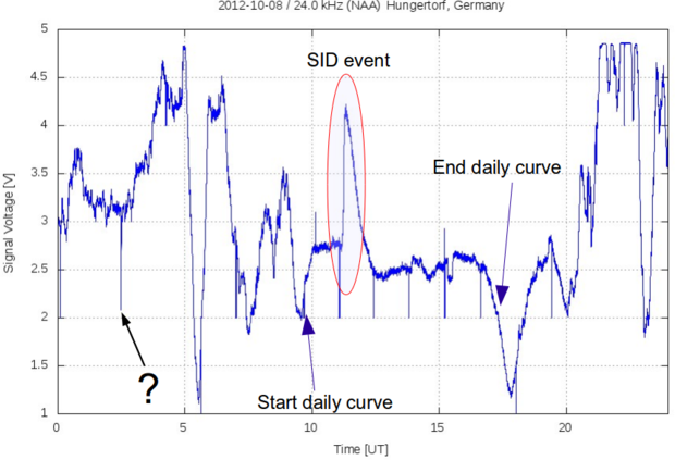
Above figure shows a typical day curve with a strong x-ray flare event around noon UTC (October 8th, 2012 measured at 24.0 kHz in Hungerstorf, northern Germany). A typical signal level plot has night time pattern, sunrise and -set pattern and a quiet day curve (QDC, which is some kind of polynomian 2nd order) where one can find SID events as an offset from this polynomian curve. Several transmitter stations have regular (weekly, daily or monthly) maintainance times. At those times random noise is dominating the plot. The spike like singularities are only seen at high temporal resolution and are not yet understood.

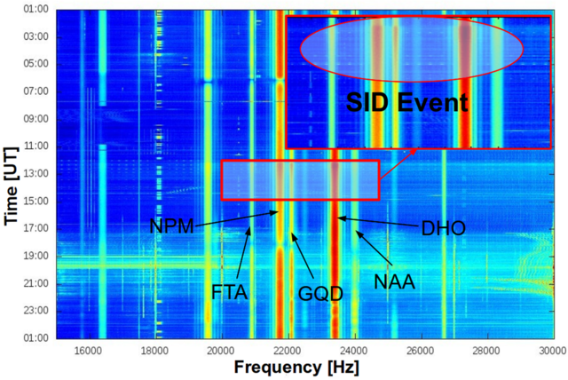
A VLF radio wave spectrum from 15 to 30 kHz is shown above. Again a disturbed day (October 8th, 2012) was choosen to demonstrate how a SID event is seen in this kind of presentation. The blown up region displays the time around noon UTC. A strong enhancement along discrete frequencies (eq. to VLF radio transmitting signal frequencies) is seen. Here it is not as straight forward to define daytime and night as well as sunrise and sunset pattern. This depends on the geographic location of the radio signal transmitter station and the receiver location. The SID monitor used here is located at northern Germany (CET time zone), but the the transmitters are from many other time zones. Find more details on the transmitter data here.

Realtime data from various InFlaMo network stations can be found at the 'Data product' site.